Ringkasan Garansi

The Company warrants that this product will be free from defects in materials and workmanship for a period of 2 years (1 year for accessories) from the date of the original purchase from the Company. Accessories such as test probes, batteries, and adapters are covered by a 1-year warranty. This limited warranty applies only to the original purchaser and is not transferable to a third party. If the product is found to be defective during the warranty period, the Company will provide repair or replacement services as described in the full warranty statement.

If a product is proven to be defective within the applicable warranty period, the Company may, at its sole discretion, either repair the defective product without charging for parts or labor, or replace the defective product with an equivalent product (as determined by the Company). Parts, modules, and replacement products provided by the Company under this warranty may be brand-new or repaired to a condition equivalent to new. All replaced parts, modules, and products shall become the property of the Company.

To receive the services covered by this warranty, the customer must notify the Company of any defects within the applicable warranty period and make appropriate arrangements for the performance of the services. The customer is responsible for packing the defective product and shipping it to the repair center designated by the Company, along with a copy of the original purchaser’s proof of purchase.

This warranty does not cover any defects, malfunctions, or damage resulting from accidents, normal wear and tear of machine parts, use outside the product’s intended scope, misuse, or improper or insufficient maintenance.

Under the terms of this warranty, the Company is not obligated to provide the following services: a) Repair damage resulting from installation, repair, or maintenance of the product by personnel other than the Company’s authorized service representatives; b) Repair of damage caused by improper use or connection to incompatible equipment; c) Repair of any damage or malfunction caused by the use of a power source not provided by the Company; d) Repair of products that have been modified or integrated with other products (if such modification or integration increases the time or difficulty required to repair the product).

Except for the warranties provided in this summary or in the applicable warranty statements, the Company makes no warranties of any kind, whether express or implied, including but not limited to implied warranties of merchantability and fitness for a particular purpose. The Company shall not be liable for any indirect, special, or consequential damages.

Daftar Isi

HYPERLINK l “_Toc25242635″2. Safety Terms and Symbols 2

HYPERLINK l “_Toc25242636″3. Quick Start 4

HYPERLINK l “_Toc25242637” An Introduction to the Structure of an Oscilloscope 4

HYPERLINK l “_Toc25242638” Front Panel 4

HYPERLINK l “_Toc25242639” Rear Panel 5

HYPERLINK l “_Toc25242640” Button Control Area 6

HYPERLINK l “_Toc25242641” An Introduction to the Oscilloscope User Interface 7

HYPERLINK l “_Toc25242642” How to Conduct a General Inspection 8

HYPERLINK l “_Toc25242643” How to Perform a Functional Test 9

HYPERLINK l “_Toc25242644” How to Perform Probe Compensation 9

HYPERLINK l “_Toc25242645” How to Set the Probe Attenuation Coefficient 10

HYPERLINK l “_Toc25242646” How to Use Probes Safely 11

HYPERLINK l “_Toc25242647” How to Perform Self-Calibration 11

HYPERLINK l “_Toc25242648” An Introduction to Vertical Systems 11

HYPERLINK l “_Toc25242649” Introduction to Leveling Systems 12

HYPERLINK l “_Toc25242650” An Introduction to Trigger Systems 13

HYPERLINK l “_Toc25242651″4. Advanced Oscilloscope User’s Guide 14

HYPERLINK l “_Toc25242652” How to Set Up a Vertical System 15

HYPERLINK l “_Toc25242653” Implementation of Mathematical Operations 16

HYPERLINK l “_Toc25242654” Dual-Waveform Calculation 16

HYPERLINK l “_Toc25242655” Using FFT17

HYPERLINK l “_Toc25242656” Applications of the Vertical Displacement Knob and Vertical Position Knob 19

HYPERLINK l “_Toc25242657” How to Set Up a Horizontal System 20

HYPERLINK l “_Toc25242658” Waveform Zoom 20

HYPERLINK l “_Toc25242659” How to Set Up Trigger 21

HYPERLINK l “_Toc25242660” Single-Touch Trigger 21

HYPERLINK l “_Toc25242661” Alternating Trigger (Edge Trigger Mode) 23

HYPERLINK l “_Toc25242662” How to Use the Function Menu 23

HYPERLINK l “_Toc25242663” How to configure data collection/display 24

HYPERLINK l “_Toc25242664” How to Save and Retrieve 25

HYPERLINK l “_Toc25242665” How to Configure Assistive System Features 31

HYPERLINK l “_Toc25242666” How to Update Instrument Firmware 33

HYPERLINK l “_Toc25242667” How to Perform Automatic Measurements 34

HYPERLINK l “_Toc25242668” How to Perform Cursor Measurements 37

HYPERLINK l “_Toc25242669” How to Use the Execute Key 39

HYPERLINK l “_Toc25242670″5. Communication with Host Computer Software42

HYPERLINK l “_Toc25242671″6. Application Examples 42

HYPERLINK l “_Toc25242672” Example 1: Measuring a Simple Signal 42

HYPERLINK l “_Toc25242673” Example 2: Measuring the Gain of an Amplifier in a Circuit 43

HYPERLINK l “_Toc25242674” Example 3: Capturing a Single Signal 44

HYPERLINK l “_Toc25242675” Example 4: Analyzing Signal Details 45

HYPERLINK l “_Toc25242676” Example 5: Applications of the X-Y Function 47

HYPERLINK l “_Toc25242677” Example 6: Video Signal Trigger 48

HYPERLINK l “_Toc25242678″7. Troubleshooting49

HYPERLINK l “_Toc25242679″8. Technical Specifications 50

HYPERLINK l “_Toc25242680″9. Appendix 54

HYPERLINK l “_Toc25242681” Appendix A: Attachment 54

HYPERLINK l “_Toc25242682” Appendix B: Daily Maintenance and Cleaning 54

Persyaratan Keselamatan Umum

Harap baca tindakan pencegahan keselamatan berikut untuk menghindari cedera pribadi dan mencegah kerusakan pada produk ini atau produk lain yang terhubung dengannya. Untuk menghindari potensi bahaya, produk ini hanya boleh digunakan dalam batas yang ditentukan.

Only qualified technicians may perform repairs.

To prevent fires or personal injury

Connect the probe correctly. The probe’s ground terminal is at ground potential. Do not connect the ground terminal to positive potential.

Use the appropriate power cord. Use only the power cord designed specifically for this product and approved for use in the country where it is being used.

Connect and disconnect properly. Do not arbitrarily connect or disconnect probes or test leads while they are connected to the power source.

Product Grounding. This product is grounded via the grounding conductor in the power cord. To prevent electric shock, the grounding conductor must be connected to earth. Before connecting to the input or output terminals of this product, ensure that it is properly grounded.
When powered by AC, this product must not be used to directly measure AC voltage, as the measurement ground is connected to the power cord’s ground; doing so may cause a power supply short circuit.

Observe all terminal ratings. To prevent the risk of fire or electric shock, pay attention to all ratings and markings on this product. Before connecting this product, read the user manual to learn more about its ratings.

Do not operate the instrument without the cover plate in place. If the cover plate or front panel has been removed, do not operate this product.

Use the appropriate fuse. Use only fuses that meet the type and rating specifications for this product.

Avoid contact with exposed circuits. Do not touch exposed contacts or components while the product is energized.

Do not operate the unit if you suspect a malfunction. If you suspect that this product is damaged, have it inspected by a qualified service technician.

Ensure adequate ventilation. Please refer to the detailed installation instructions in the user manual to install this product correctly and ensure adequate ventilation.

Do not operate in a damp environment.

Do not operate in flammable or explosive environments.

Jaga agar permukaan produk tetap bersih dan kering.

Safety Terms and Symbols

Ketentuan Keselamatan
: Terms used in this manual. The following terms may appear in this manual:

Warning: Warning statements indicate situations or operations that may pose a risk to life.

Note: This cautionary statement identifies situations or operations that may result in damage to this product or other property.

Terms on the product. The following terms may appear on the product:

Danger: Indicates that performing this action may result in immediate harm to you.

Warning: This indicates that performing this action may pose a potential risk to you.

Note: This indicates that performing this action may cause damage to this product or other devices connected to it.

Simbol Keamanan

Symbols on the product. The following symbols may appear on the product:

High Voltage Caution Protective Ground Terminal Enclosure Ground Terminal Measurement Ground Terminal

Please refer to the manual

Harap baca tindakan pencegahan keselamatan berikut untuk menghindari cedera pribadi dan mencegah kerusakan pada produk ini atau produk lain yang terhubung dengannya. Untuk menghindari potensi bahaya, produk ini hanya boleh digunakan dalam batas yang ditentukan.

Peringatan:

The two channels of the oscilloscope are non-isolated. Be sure to use a common reference for both channels during measurements. Do not connect the ground wires of the two probes to two different non-isolated DC potentials; otherwise, a short circuit may occur due to the ground connections of the oscilloscope probes.

Peringatan:

Be sure to use a common reference for the channels during measurement; otherwise, a short circuit may occur due to the ground connection of the oscilloscope probe.

Schematic Diagram of Internal Ground Connections in an Oscilloscope:

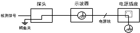
When an AC-powered oscilloscope is connected via a port to an AC-powered computer, the primary-side power supply of the utility grid cannot be measured.

Warning: When the input ports are connected to a circuit with a peak voltage exceeding 42 V (30 Vrms) or a power rating exceeding 4800 VA, to avoid electric shock or fire: Use only the appropriately insulated voltage probes and test leads supplied with the oscilloscope, or accessories specified by the manufacturer as suitable for this series of oscilloscopes. Before use, inspect the oscilloscope probes and accessories for mechanical damage; if any damage is found, replace them. Remove all unused test probes, probes, and accessories. Disconnect the computer communication cable. Do not use an input voltage higher than the instrument’s rating. Exercise particular caution when using 1:1 test leads, as the probe voltage is directly transmitted to the oscilloscope. Do not touch exposed metal BNC connectors. Do not insert metal objects into the connectors.

Ringkas

Oscilloscope Model Correspondence Chart

LISUN Pilih Model	Saluran	Bandwidth	Tingkat Sampling	Resolusi Vertikal	Ukuran Layar
OSP1102	Saluran Ganda	100M	1G	8 bit	7 inci
OSP3202E	Saluran Ganda	200M	1G	8 bit	8 inci
OSP3302	Saluran Ganda	300M	2.5G	8 bit	8 inci
OSP3202A	Saluran Ganda	200M	2.5G	14 bit	8 inci
OSP3104E	Empat saluran	100M	1G	8 bit	8 inci
OSP104AE	Empat saluran	100M	1G	14 bit	8 inci
OSP3204E	Empat saluran	200M	1G	8 bit	8 inci
OSP3204AE	Empat saluran	200M	1G	14 bit	8 inci

An Introduction to the Structure of an Oscilloscope

This chapter provides a brief description and introduction to the operations and functions of the oscilloscope’s front panel, enabling you to become familiar with using the oscilloscope in the shortest possible time.

Panel depan

The oscilloscope panel includes knobs and function keys. On the right side of the display, there are five keys that serve as menu selection keys. You can use them to configure various options in the current menu. The other keys are function keys, which allow you to access different function menus or directly access specific functions.

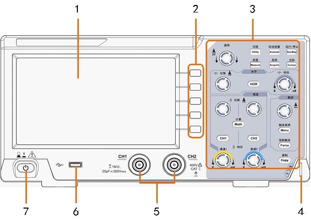
Figure 3 Figure 1: Oscilloscope Front Panel

Tampilan di Area

Menu Selection Button: Selects menu items on the right-hand screen.

Button and Knob Control Area

Probe compensation: 5V/1 kHz signal output.

Signal Input Port

USB Host Port: This port is used to transfer data when the oscilloscope is connected to an external USB device as the “host.” For example, this port is used when saving waveforms to a USB flash drive.

Oscilloscope Switch

Panel belakang

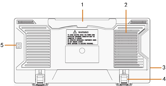
Figure 3, Figure 2: Rear Panel of the Oscilloscope

Pegangan yang dapat ditarik

Lubang ventilasi

Stopkontak

Stand: Allows you to adjust the angle of the oscilloscope.

USB Device Port: This port is used to transfer data when the oscilloscope is connected to an external USB device as a “slave device.” For example, use this port when connecting to a PC.

Area Kontrol Tombol

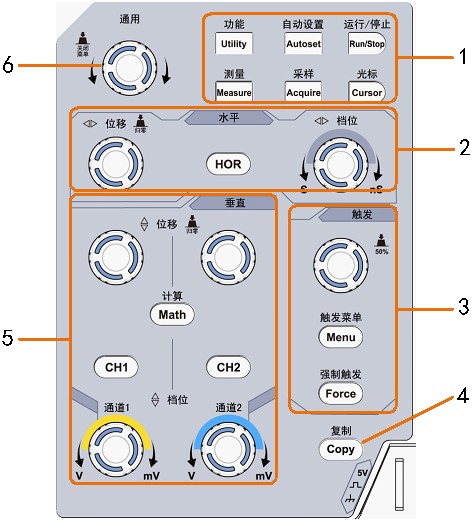
Figure 3: Diagram of the Button and Knob Control Area

Function Key Area: 6 keys in total.

Level Control Zone:

It includes one button and two knobs.

The “HOR” button accesses the horizontal system settings menu; the “Horizontal Shift” knob controls the horizontal shift when triggered; and the “Horizontal Step” knob controls the time base step size.

Trigger Control Zone:

It includes two buttons and a knob.

The “Trigger Level” knob adjusts the trigger level. The other two buttons correspond to the trigger system settings.

Copy Key: This key serves as a shortcut for the “Save” function in the Function Panel’s function menu. Pressing this key is equivalent to selecting “Save” from the Save menu. It saves waveforms, settings, or screen images based on the save type selected in the Save menu.

Vertical Control Zone:

It includes three buttons and four knobs.

The “CH1” and “CH2” buttons correspond to the setup menus for Channel 1 and Channel 2, respectively, while the “Math” button corresponds to the waveform calculation menu, which includes operations such as addition, subtraction, multiplication, division, and FFT. The two “Vertical Offset” knobs control the vertical offset for Channel 1 and Channel 2, respectively. The two “Range” knobs control the voltage ranges for Channel 1 and Channel 2, respectively.

Universal Knob: When the icon appears in the on-screen menu, it indicates that you can turn the Universal Knob to select the current menu or adjust a setting; pressing the knob closes the menus on the left and right sides of the screen.

An Introduction to the Oscilloscope User Interface

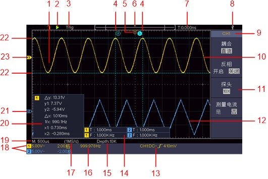
Fig. 3 and Fig. 4: Illustrations of the display interface

1. Waveform display area.

2. Start/Stop.

3. The trigger status indicator includes the following types of information:

Auto: The oscilloscope is in Auto mode and is capturing waveforms without a trigger.

Trig: The oscilloscope has detected a trigger and is now acquiring post-trigger data.

Ready: All pre-trigger data has been acquired, and the oscilloscope is ready to accept a trigger.

Scan: The oscilloscope continuously acquires and displays waveform data in scan mode.

Stop: The oscilloscope has stopped acquiring waveform data.

4. The two vertical blue dashed lines indicate the vertical position of the cursor as measured by the cursor.

5. The T pointer indicates the trigger horizontal displacement; its position can be adjusted using the horizontal displacement control knob.

6. The pointer indicates the trigger position within the current storage depth.

7. Indicates the value that currently triggers horizontal displacement. Displays the current waveform window’s position in memory.

8. Indicates that a USB flash drive is currently inserted into the oscilloscope.

9. Channel identifier for the current menu

10. Waveform for Channel 1.

11. Right-side screen menu.

12. Waveform for Channel 2.

13. The icon indicates the trigger type selected for the corresponding channel:

Rising-edge-triggered video line synchronization

Falling-edge-triggered video field synchronization trigger

The reading indicates the trigger level for the corresponding channel.

14. Display the measurement parameters and values for the corresponding channel. Here, T denotes the period, F denotes the frequency, V denotes the average value, Vp denotes the peak-to-peak value, Vr denotes the root mean square (RMS) value, Ma denotes the maximum value, Mi denotes the minimum value, Vt denotes the top value, Vb denotes the bottom value, Va denotes the amplitude, Os denotes overshoot, Ps denotes pre-shoot, RT denotes rise time, FT denotes fall time, PW denotes positive pulse width, NW denotes negative pulse width, +D denotes positive duty cycle, -D denotes negative duty cycle, PD denotes delay A-> B, ND denotes delay A-> B, TR denotes cycle-to-cycle RMS, CR denotes cursor RMS, WP denotes on-screen pulse width ratio, RP denotes phase, +PC denotes the number of positive pulses, -PC denotes the number of negative pulses, +E denotes the number of rising edges, -E denotes the number of falling edges, AR denotes area, and CA denotes cycle area.

15. Current storage depth.

16. The trigger frequency display shows the frequency of the signal on the corresponding channel.

17. Current Sampling Rate

18. The readings indicate the voltage range and zero point for the corresponding channel, respectively. BW indicates the bandwidth limit.

The icon indicates the channel’s coupling mode:

“—” indicates DC coupling

“～” indicates AC coupling

“” indicates a ground-coupled reading

19. The reading indicates the set value of the main clock.

20. Cursor Measurement Window: Displays the absolute values of the cursors and the readings for each cursor.

21. The blue pointer indicates the ground reference point (zero position) of the waveform displayed on Channel CH2. If there is no pointer indicating a channel, it means that channel is not enabled.

22. The two horizontal blue dashed lines indicate the horizontal cursor positions measured by the cursor.

23. The yellow pointer indicates the ground reference point (zero position) for the waveform displayed on Channel 1 (CH1). If there is no pointer indicating a channel, it means that channel is not enabled.

How to Conduct a General Examination

When you receive a new oscilloscope, we recommend that you follow these steps to inspect the instrument.

1. Check for any damage caused by shipping.

If you find that the shipping carton or foam padding is severely damaged, please set it aside until the unit and its accessories have passed electrical and mechanical testing.

2. Check the attachments.

Details regarding the included accessories are provided in “Appendix A: Accessories” of this manual. Please refer to this section to check for any missing accessories. If you find that any accessories are missing or damaged, please contact our authorized dealer responsible for this product or our local office.

3. Inspect the entire unit.

If you notice any damage to the instrument’s exterior, if the instrument is not functioning properly, or if it fails performance testing, please contact the Company’s authorized dealer responsible for this business or the Company’s local office. If the instrument is damaged during shipping, please be sure to retain the packaging. Notify the shipping department and the Company’s authorized dealer responsible for this business. The Company will arrange for repair or replacement.

How to Perform a Functional Test

Perform a quick functional check to verify that this instrument is operating normally. Please follow these steps:

1. Turn on the instrument by pressing the power button located at the bottom left of the main unit.
You will hear a faint clicking sound from the internal relay. The instrument will perform all self-tests, and the startup screen will appear. Press the “Utility” button on the front panel, select the “Function” menu item on the right, select “Calibration” from the left-hand function menu, and then select “Factory Settings” from the right-hand menu. The default attenuation factor setting in the probe menu is 10X.

2. Set the switch on the oscilloscope probe to 10X, and connect the probe to CH1.

Align the slot on the probe with the plug on the CH1 connector’s coaxial cable fitting (BNC), insert it, then rotate the probe to the right and tighten it.

Connect the probe tip and the ground clip to the connector on the probe compensator.

3. Press the “Auto Setup” button on the front panel.

Within a few seconds, a square wave will appear on the display (1 kHz frequency, 5 V peak-to-peak), as shown in Figure 35.

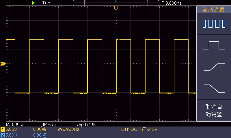
Fig. 3–Fig. 5: Automatic Settings

Repeat steps 2 and 3 to test the CH2 channel.

How to Perform Probe Compensation

Perform this adjustment the first time you connect the probe to any input channel to match the probe to the input channel. Probes that are not compensated or have compensation deviations can cause measurement errors or inaccuracies. To adjust the probe compensation, follow these steps:

Set the probe menu attenuation factor to 10X, set the switch on the probe to 10X (see “How to Set the Probe Attenuation Factor” on page 10), and connect the oscilloscope probe to channel CH1. If using a hook-type probe tip, ensure that it makes firm contact with the probe. Connect the tip of the probe to the signal output connector on the probe compensator, connect the reference lead clip to the ground connector on the probe compensator, and then press the Auto Setup button on the front panel.

Examine the displayed waveform and adjust the probe until the compensation is correct. See Figures 36 and 37.

Compensation, Overcompensation, Correct Compensation, Undercompensation

Figure STYLEREF 1 s3SEQ Figure * ARABIC s 16: Probe Compensation Waveform Display

Repeat the steps if necessary.

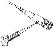
Figure STYLEREF 1 s3SEQ Figure * ARABIC s 17: Probe Adjustment

How to Set the Probe Attenuation Coefficient

Probes have various attenuation factors, which affect the vertical scale factor of the oscilloscope.

To change (or check) the probe attenuation factor setting in the oscilloscope menu, follow these steps:

Press the function menu button corresponding to the channel you are using (the CH1 button or the CH2 button).

Select “Probe” from the menu on the right, then turn the “General” knob to select the desired attenuation factor from the menu on the left. This setting remains in effect until it is changed again.

Note: The probe attenuation factor in the oscilloscope’s menu is factory-set to 10X. Make sure the setting on the probe’s attenuation switch matches the probe attenuation factor option in the oscilloscope’s menu.

The probe switch has settings of 1X and 10X. See Figure 38.

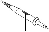
Figure 3, Figure 8: Probe Attenuation Switch

Note: When the attenuation switch is set to 1X, the probe limits the oscilloscope’s bandwidth to 5 MHz. To use the oscilloscope’s full bandwidth, be sure to set the switch to 10X.

How to Use the Probe Safely

The safety ring surrounding the probe body provides a barrier that prevents fingers from receiving an electric shock. See Figure 39.

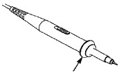
Figure 3, Figure 9: Probe Finger Safety Ring

Warning: To prevent electric shock when using the probe, keep your fingers behind the safety ring on the probe body. To prevent electric shock when using the probe, do not touch the metal parts of the probe tip while the probe is connected to a voltage source. Before taking any measurements, connect the probe to the instrument and connect the ground terminal to earth.

How to Perform Self-Calibration

The self-calibration procedure quickly brings the oscilloscope to its optimal state to ensure the most accurate measurements. You can run this procedure at any time, but you must run it whenever the ambient temperature changes by 5°C or more.

To perform an auto-calibration, disconnect all probes or leads from the input connector. Then, press the Utility key, select “Functions” from the right-hand menu, select “Calibration” from the left-hand menu, select “Auto-calibration” from the right-hand menu, and confirm that you are ready before proceeding.

An Introduction to Vertical Systems

As shown in Figure 310, there is a series of buttons and knobs in the Vertical control area. The exercises below will gradually guide you through using the vertical settings.

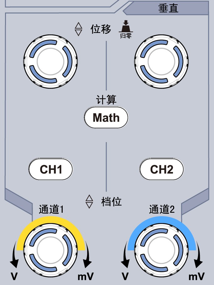
Figure 3, Figure 10: Vertical Control Zone

Use the Vertical Offset knob to center the signal in the waveform window. The Vertical Offset knob controls the vertical display position of the signal. When you turn the Vertical Offset knob, the pointer indicating the channel’s ground reference point moves up and down with the waveform.

Teknik Pengukuran

If the channel coupling mode is DC, you can quickly measure the DC component of the signal by observing the gap between the waveform and the signal ground.

If the coupling mode is AC, the DC component in the signal is filtered out. This mode allows you to display the AC component of the signal with higher sensitivity.

Shortcut key to reset vertical displacement to zero in dual analog channels

Rotate Vertical Position: This knob not only allows you to adjust the vertical display position of a channel, but you can also press it to reset the channel’s vertical display position to zero.

Change the vertical settings and observe the resulting changes in the status information.

You can determine changes in the vertical scaling factor for any channel based on the information displayed in the status bar below the waveform window.

Turn the Vertical Scale knob to change the vertical scale factor (voltage scale), and you will notice that the scale factor displayed in the status bar for the corresponding channel changes accordingly.

Press the CH1, CH2, and Math buttons to display the operation menu, indicators, waveforms, and range factor status information for the corresponding channels on the screen.

Introduction to Leveling Systems

As shown in Figure 311, there is one button and two knobs in the Horizontal Control section. The exercises below will gradually guide you through the process of setting the horizontal time base.

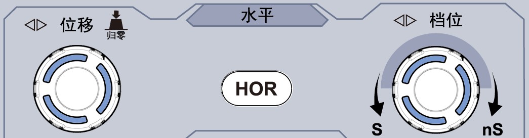
Figure 3, Figure 11: Horizontal Control Zone

Turn the “Horizontal Time Base” knob to change the horizontal time base setting and observe the resulting changes in the status information. As you turn the “Horizontal Time Base” knob to adjust the horizontal time base, you will notice that the display in the status bar corresponding to the “Horizontal Time Base” changes accordingly.

Rotate the Horizontal Offset knob to adjust the horizontal offset of the signal in the waveform window.

Horizontal Displacement: The Horizontal Displacement knob controls the horizontal displacement of the signal. When you turn the Horizontal Displacement knob, you can observe the waveform moving horizontally in response to the knob’s rotation.

Shortcut key to reset trigger point offset to the horizontal zero point

Horizontal Offset: The knob not only allows you to adjust the horizontal offset of the signal in the waveform window by turning it, but you can also press it to reset the trigger offset to the horizontal zero point.

Press the HOR button to toggle between Normal Mode and Waveform Zoom Mode.

An Introduction to Trigger Systems

As shown in Figure 312, the Trigger Control Area contains one knob and two buttons. The exercises below will gradually guide you through the settings of the trigger system.

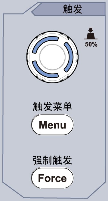
Figure 3, Figure 12: Trigger Control Zone

Press the “Trigger Menu” button to bring up the trigger menu. You can change the trigger settings by selecting the appropriate button options from the menu.

Use the “Trigger Level” knob to change the trigger level setting.

Turn the “Trigger Level” knob, and you will see the trigger pointer on the screen move up and down as you turn the knob. As the trigger pointer moves, you will notice that the trigger level value displayed on the screen changes.

Note: Turning the “Trigger Level” knob not only changes the trigger level value, but also serves as a shortcut to set the trigger level to the midpoint of the trigger signal amplitude when the knob is pressed.
Press the “Force Trigger” button to force the generation of a trigger signal; this is primarily used in the “Normal” and “Single” modes of the trigger settings.

4. Advanced User Guide for the Oscilloscope This chapter covers the following topics: • How to configure the vertical system • How to configure the horizontal system • How to configure triggering • How to configure data acquisition and display • How to save and recall settings • How to configure auxiliary functions • How to Update Instrument Firmware • How to Perform Automatic Measurements • How to Perform Cursor Measurements • How to Use the Execution Key

We recommend that you read this chapter carefully to familiarize yourself with the oscilloscope’s various measurement functions and other operating procedures.

How to Set Up a Vertical System

The vertical system control section includes three menu buttons—CH1, CH2, and Math—and four knobs: vertical displacement and vertical range (one set for each of the two channels).

Configuration of Channel 1 and Channel 2

Each channel has its own vertical menu. Each item is configured separately for each channel.

How to Turn Waveforms On or Off (Channels, Waveform Calculations)

Pressing the CH1, CH2, or Math front-panel button will produce the following results:

If the waveform is closed, open it and display its menu.

If the waveform is open but its menu is not displayed, display its menu.

If the waveform is open and its menu is displayed, closing the waveform will also cause the menu to disappear.

See the table below for a description of the channel menu:

Function Menu	Pengaturan	Note
Kopel	DC, AC, Grounding	Through the AC and DC components of the input signal. Block the DC component of the input signal. Disconnect the input signal.
Terbalik	Turn On Turn Off	Enable the waveform inversion function. The waveform is displayed normally.
Penyelidikan	1X 10X 100X 1000X	Select one of the values based on the probe attenuation factor to ensure accurate vertical scale readings.
Mengukur Arus	Ya atau tidak	Select “Yes” if you are measuring current based on the voltage drop across the resistor using a Voltage Probe.
A/V or mA/V (displayed when current measurement is selected)	V/A or mV/A	Turn the universal knob to set the ampere-to-volt ratio; the adjustable range is 100 mA/V to 1 kA/V. The ampere-to-volt ratio equals 1 divided by the resistance value. The volt-to-ampere ratio is calculated automatically.
Bandwidth Limitation (Available only on the NDS1102S and NDS1202S)	Total bandwidth: 20M	Oscilloscope Bandwidth: Limit the bandwidth to 20 MHz to reduce display noise.

Set Channel Coupling

Taking Channel 1 as an example, the signal under test is a square wave with a DC offset. The procedure is as follows:

Press the CH1 button to bring up the CH1 settings menu.

In the right-hand menu, press “Coupling” to switch to “DC” and set the coupling mode to DC. Both the DC and AC components of the signal under test will be passed through.

In the right-hand menu, press “Coupling” to switch to “AC” and set the coupling mode to AC. The DC component in the signal under test is blocked.

Set Waveform Inversion

Waveform Inversion: The displayed signal is inverted by 180 degrees relative to ground potential.

Taking Channel 1 as an example, the steps are as follows:

Press the CH1 button to bring up the CH1 settings menu.

In the menu on the right, select “Invert” and set it to “On” to enable the waveform inversion feature. Then select “Invert” again and set it to “Off” to disable the waveform inversion feature.

Adjust the Probe Scale

To match the probe’s attenuation factor, you need to adjust the probe attenuation ratio accordingly in the channel operation menu (see “How to Set the Probe Attenuation Factor” on page 10). If the probe attenuation ratio is 1:1, the oscilloscope’s input channel should also be set to 1X to prevent errors in the displayed range factor and measured data.

Taking Channel 1 as an example, with a probe attenuation factor of 10:1, the procedure is as follows:

Press the CH1 button to bring up the CH1 settings menu.

In the right-hand menu, select “Probe.” In the left-hand menu, turn the “General” knob to 10X.

Measure the current by measuring the voltage drop across the resistor using the Voltage Probe

Taking Channel 1 as an example, if you want to measure current by measuring the voltage drop across a 1Ω resistor using the Voltage Probe, follow these steps:

Press the CH1 button to bring up the CH1 settings menu.

In the right-hand menu, set “Measure Current” to “Yes”; the A/V ratio menu item will appear below. Select this menu item, then turn the General knob to set the ampere-to-volt ratio. The ampere-to-volt ratio equals 1 divided by the resistance value. Here, the A/V ratio is set to 1.

Implementation of Mathematical Operations

The Math function displays the results of adding, subtracting, multiplying, or dividing the waveforms of Channel 1 and Channel 2, or performing a Fourier transform on a specific channel. Press the Math key to display the waveform calculation menu on the right.

Double-Waveform Calculation

Press the Math key to display the waveform calculation menu on the right; press Type to switch to dual-waveform calculation.

Function Menu	Pengaturan	Note
Tipe	Double-Waveform Calculation	Display the Dual Waveform Calculation Menu
Faktor 1	CH1 CH2	Select a signal source with a factor of 1
Символ	+ – * /	Select an operator
Faktor 2	CH1 CH2	Select a signal source with a factor of 2
Halaman berikutnya		Go to the Next Page Menu
Vertical (Grid)		Rotate the universal knob to adjust the vertical position of the Math waveform
Vertical (V/cell)		Turn the universal knob to adjust the voltage range of the Math waveform.
Halaman Sebelumnya		Back to the Previous Page Menu

Taking Channel 1 + Channel 2 as an example, the steps are as follows:

Press the Math button to display the waveform calculation menu on the right side of the screen; the pink waveform M appears on the screen.

In the menu on the right, select “Type” as “Dual-Waveform Calculation.”

In the menu on the right, select CH1 as Factor 1.

In the menu on the right, select the + symbol.

In the menu on the right, select “Factor 2” as “CH2.”

In the right-hand menu, select “Next Page,” then select “Vertical (Grid)” to position the marker on this menu item, and rotate the “General” knob to adjust the vertical position of the Math waveform.

Select “Vertical (V/Grid)” from the menu on the right to position the marker on this menu item, then turn the “General” knob to adjust the voltage range of the Math waveform.

Using FFT

FFT breaks down a signal into its component frequencies, and the oscilloscope uses these component frequencies to display a graph of the signal in the frequency domain, as opposed to the oscilloscope’s standard time-domain graph. These frequencies can be matched to known system frequencies, such as the system clock, an oscillator, or the power supply.

This oscilloscope’s FFT function converts 2048 data points from a time-domain waveform into a frequency-domain signal. The resulting FFT spectrum contains 1024 points ranging from DC (0 Hz) to the Nyquist frequency.

Press the Math button to display the waveform calculation menu on the right; press Type to switch to FFT.

Function Menu	Pengaturan	Note
Tipe	FFT	Display the FFT menu
sumber	CH1 CH2	A waveform on which the corresponding Fourier transform has been performed
Jendela	Hamming, Rectangle, Blackman, Hanning, Kaiser, Bartlett	Turn the general knob to select the window function from the left-hand menu.
Orientasi	Vrms dB	Set the format to Vrms. Set the format to dB.
Halaman berikutnya		Go to the next page’s menu
Frekuensi (Hz)	Frequency Frequency/Cell	To change the horizontal position or horizontal time base of the selected FFT waveform, turn the M knob to adjust it.
Vertikal	V or dBVrms	To change the vertical position or voltage range of the selected FFT waveform, turn the M knob to adjust it.
Halaman Sebelumnya		Back to the Previous Page Menu

Using the Fourier transform as an example, the steps are as follows:

Press the Math button to display the waveform calculation menu on the right; a pink waveform labeled “M” appears on the screen.

In the menu on the right, select “FFT” for “Type.”

In the menu on the right, select “Source” and switch to CH1.

Select “Window” from the menu on the right, and in the menu on the left, turn the “General” knob to select the type of window you want to use.

In the menu on the right, select “Format” as Vrms or dB.

In the right-hand menu, press “Horizontal (Hz)” to position the marker before the frequency value, then turn the “General” knob to adjust the horizontal position of the FFT waveform; next, press again to position the marker below “Frequency/Div,” and turn the “General” knob to adjust the horizontal time base of the FFT waveform.

Select “Vertical” from the menu on the right, and follow the same steps as above to set the vertical position and voltage level.

Select an FFT Window

The FFT function provides six windows. Each window strikes a balance between frequency resolution and amplitude accuracy. The characteristics of the object being measured and the source signal help determine which window to use. Use the following principles to select the most appropriate window.

Jenis Jendela	Note	Jendela
Hamming	This is the optimal window type for resolution frequencies that are very close to the same value, and it offers slightly better amplitude accuracy than the “rectangular” window. The Hamming window offers slightly higher frequency resolution than the Hanning window. Use the Hamming window to measure sinusoidal, periodic, and narrowband random noise. This window is used for transients or bursts occurring before or after events with significant differences in signal level.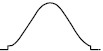
empat persegi panjang	This is the best window type for resolution frequencies that are very close to the same value, but it performs the worst when accurately measuring the amplitude of these frequencies. It is the best choice for measuring the spectrum of non-repeating signals and for measuring frequency components close to DC. Use the “rectangular” window to measure signal levels in transients or bursts that occur immediately before or after events with nearly identical frequencies. In addition, this window can be used to measure sine waves of equal amplitude with very closely spaced frequencies, as well as broadband random noise with relatively slow spectral variations.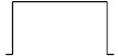
Pria kulit hitam	This type of window is best suited for measuring frequency amplitude, but it is the least effective for measuring frequency resolution. Use the Blackman window to identify the primary single-signal frequency waveform from which higher-order harmonics are derived.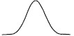
hanning	This type of window provides excellent amplitude accuracy but is less effective for frequency resolution. Use the Hanning window to measure sinusoidal, periodic, and narrowband random noise. This window is used for transients or bursts occurring before or after events with significant differences in signal level.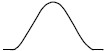
Kaiser	When using the Kaiser window, the frequency resolution is average, but spectral leakage and amplitude accuracy are both good. The Kaiser window is best suited for situations where frequencies are very close to one another but the amplitudes differ significantly (with side-lobe levels and shape factors closest to those of the traditional Gaussian RBW). This window is also well-suited for random signals.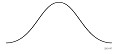
Bartlett	The Bartlett window is very similar to the triangular window (with zeros at both ends).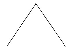

FFT Tips and Tricks

Use the default dB scale to view a detailed representation of multiple frequencies, even if their amplitudes vary significantly. Use the Vrms scale to view an overall representation that allows for comparison across all frequencies.

Signals containing a DC component or offset can cause errors or deviations in the FFT spectrum components. To reduce the DC component, you can select the AC coupling mode.

To reduce random noise from repetitive or single-pulse events, as well as aliasing frequency components, you can set the oscilloscope’s acquisition mode to average acquisition.

Definisi:

Nyquist frequency: The highest frequency that any real-time digital oscilloscope can measure without error is half the sampling rate. This frequency is called the Nyquist frequency. Frequency information above the “Nyquist” frequency is undersampled, which can result in FFT aliasing. When using FFT, attention should be paid to the ratio of the sampling rate to the measured frequency.

Applications of the Vertical Displacement Knob and the Vertical Position Knob

1. Vertical Offset: Use the knob to adjust the vertical offset of the waveform for the corresponding channel.

The resolution of this control knob varies depending on the vertical setting.

2. Vertical Scale: Use the knob to adjust the vertical resolution of the waveform for the corresponding channel.

Determine the vertical sensitivity in 1–2–5-step increments.

The lower-left corner of the screen displays vertical displacement and vertical channel information. See Figure 41.

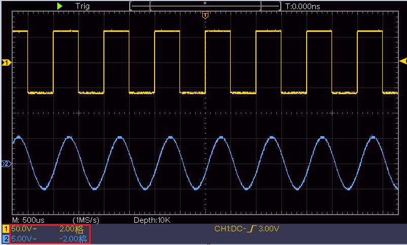
Figure 4 Figure 1: Vertical Displacement Data

How to Set Up a Leveling System

The horizontal control section includes the HOR button, the horizontal movement knob, and the horizontal position knob.

Horizontal Offset Knob: Adjusts the horizontal offset for all channels (including mathematical operations); the resolution of this knob varies depending on the time base.

Horizontal Scale Knob: Sets the horizontal scale factor for the main window or the zoom window.

HOR Key: Toggles between Normal Mode and Waveform Zoom Mode. See the section below for details on Waveform Zoom.

Waveform Zoom

Press the HOR button to enter waveform zoom mode. The upper half of the display shows the main window, and the lower half shows the zoom window. The zoom window is an enlarged view of the selected area in the main window.

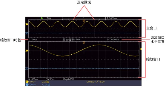
In Normal mode, the Horizontal Displacement knob and the Horizontal Scale knob can be used to adjust the horizontal position and horizontal time base of the main window.

In waveform zoom mode, the Horizontal Shift knob and the Horizontal Scale knob can be used to adjust the horizontal position and horizontal time base of the zoom window.

How to Set Up a Trigger

The trigger determines when the oscilloscope begins acquiring data and displaying waveforms. Once the trigger is set correctly, it can transform an unstable display into a meaningful waveform.
When the oscilloscope begins data acquisition, it first collects enough data to plot the waveform to the left of the trigger point. The oscilloscope continuously acquires data while waiting for the trigger condition to occur. Once the trigger is detected, the oscilloscope continuously acquires enough data to plot the waveform to the right of the trigger point.

The control panel includes a knob and two function menu buttons.

Trigger Level: Trigger Level Adjustment Knob—rotate this knob to set the signal voltage corresponding to the trigger point; press this knob to center the trigger level at the midpoint of the trigger signal amplitude.

Force Trigger: A force trigger button that forces the generation of a trigger signal; it is primarily used in the “Normal” and “Single” modes of the trigger settings.

Trigger Menu: The button that activates the menu.

Kontrol Pemicu

There are two types of triggering: single-touch and alternate. Each type uses a different function menu.

Single-Touch Triggering: Captures data from both channels simultaneously using a user-defined trigger signal to achieve stable, synchronized waveforms.

Alternating Trigger: Stabilizes asynchronous signals.

The following sections explain the “Single-Touch Trigger” and “Alternating Trigger” menus, respectively.

Single-touch activation

There are two modes for single-touch triggering: edge triggering and video triggering.

Edge-triggered: An edge-triggered event occurs when a trigger input passes through a given voltage level in a specified direction.

Video Trigger: Applies field or line video triggering to a standard video signal.

The following explains the two trigger modes for single-touch triggering.

1. Edge Triggering

Edge triggering occurs at the trigger level of the input signal’s edge. When “Edge Trigger” is selected, triggering occurs on the rising or falling edge of the input signal.
Press the Trigger Menu button to display the trigger mode menu on the right side of the screen. Press the Trigger Type menu item to switch to Single Trigger. Press the “Single Trigger Type” menu item to switch to “Edge.”
The trigger settings are displayed in the lower-right corner of the screen; for example, this indicates that the trigger type is “Edge,” the trigger source is “CH1,” the trigger coupling is “DC,” and the trigger level is “0.00 mV.”

The edge-triggered menu is described in the table below:

Function Menu	Pengaturan	Note
Tipe Pemicu	Satu sentuhan	Set the trigger type for the vertical channel to “single touch.”
Single-touch type	Tepi	Set the single-touch type for the vertical channel to edge-triggered.
sumber	CH1 CH2	Set Channel 1 as the source trigger signal. Set Channel 2 as the source trigger signal.
mode	Otomatis, Normal, Tunggal	Set the instrument to acquire waveforms even when no trigger conditions are detected. Set the instrument to acquire waveforms only when trigger conditions are met. Set the instrument to sample a single waveform when a trigger is detected, and then stop.
Halaman berikutnya		Go to the next page’s menu
Kopel	ACDC	Set to block the DC component. Set to allow all components to pass.
Lereng		Set to trigger on the rising edge of the signal. Set to trigger on the falling edge of the signal.
Explanation of “Yi”		100 ns to 10 s; use the general-purpose knob to adjust the time interval for the restart trigger circuit.
Release and Reset		Set the trigger release time to 100 ns
Halaman Sebelumnya		Back to the Previous Page Menu

Trigger Level: The trigger level indicates the vertical trigger position of the channel. Turn the Trigger Level knob to adjust the trigger level value. During the setup process, a dashed line appears to show the trigger level position, and the trigger level value in the lower-right corner changes accordingly. Once setup is complete, the dashed line disappears.

2. Video Trigger

Video triggering can be set to trigger on a field or line of an NTSC, PAL, or SECAM standard video signal.
Press the Trigger Menu button to display the trigger mode menu on the right side of the screen. Press the Trigger Type menu item to switch to Single Trigger. Press the Single Trigger Type menu item to switch to Video. Trigger settings are displayed in the lower-right corner of the
screen; for example, this indicates that the trigger type is Video, the trigger source is CH1, and the sync type is Field. The
Video Trigger menu is described in the table below:

Function Menu	Pengaturan	Note
Tipe Pemicu	Satu sentuhan	Set the trigger type for the vertical channel to “Single Touch.”
Single-touch type	Video	Set the trigger type for the vertical channel to “Video Trigger”
sumber	CH1 CH2	Set Channel 1 as the source trigger signal. Set Channel 2 as the source trigger signal.
Standar	NTSC, PAL, SECAM	Set the video format standard.
Halaman berikutnya		Go to the next page’s menu
Sinkronkan	Row, Field, Odd Field, Even Field, Specified Row	Set synchronization to trigger on a video line. Set synchronization to trigger on a video field. Set synchronization to trigger on an odd video field. Set synchronization to trigger on an even video field. Set synchronization to trigger on a specified video line. Select the “Specified Line” menu item and turn the “General” knob to set the line number.
Halaman Sebelumnya		Back to the Previous Page Menu

Alternating Trigger (Trigger Mode: Edge)

In alternate triggering, the trigger signals come from two vertical channels. This method can be used to observe two uncorrelated signals simultaneously. The trigger mode is fixed as edge triggering.
The menu description for alternate triggering (with edge trigger mode) is as follows:

Function Menu	Pengaturan	Note
Tipe Pemicu	Bergantian	Set the trigger type for the vertical channel to “Alternate.”
sumber	CH1 CH2	Set Channel 1 as the source trigger signal. Set Channel 2 as the source trigger signal.
Halaman berikutnya		Go to the next page’s menu
Kopel	ACDC	Set to block the DC component. Set to allow all components to pass.
Lereng		Set to trigger on the rising edge of the signal. Set to trigger on the falling edge of the signal.
Explanation of “Yi”		100 ns to 10 s; use the general-purpose knob to adjust the time interval for the restart trigger circuit.
Release and Reset		Set the trigger release time to 100 ns
Halaman Sebelumnya		Back to the Previous Page Menu

How to Use the Function Menu

The function menu control area includes four function menu buttons—Function, Measure, Sample, and Cursor—as well as two immediate-execution buttons—Auto Setup and Run/Stop.

How to Configure Sampling/Display Press the “Sampling” button. The descriptions for the sampling and display settings in the right-hand menu are as shown in the table below:

Function Menu	Pengaturan	Note
Collection Mode	Sampling, Peak Detection, Average	Standard Sampling Mode: Used to detect interference glitches and reduce the likelihood of confusion. Used to reduce random and irrelevant noise in the signal. Turn the “General” knob in the left-hand menu to select an averaging count of 4, 16, 64, or 128.
Tipe	Point Vector	Displays only the sample points. Vector fill displays the space between adjacent sample points.
Perasaan senang sesudah mengalami kesenganan	Close 1 second 2 seconds 5 seconds Forever	Pilih durasi.
XY Mode	Turn On Turn Off	Turn XY Mode On/Off
Hardware Frequency	Turn On Turn Off	Turn the Hardware Frequency Counter On/Off

Afterglow:
When the afterglow feature is enabled, it simulates the afterglow display of a CRT oscilloscope, with the colors of the retained raw data fading gradually while the colors of new data appear brighter.
(1) Press the “Sample” button on the panel.
(2) In the menu on the right, press “Afterglow” to select different durations: “Off,” “1 second,” “2 seconds,” “5 seconds,” and “Infinite.” When the duration is set to “Infinite,” the recorded points remain on the screen until the control value is changed. Select “Off” to turn off the afterglow and clear the display.

XY Mode:
When XY mode is selected, both Channel 1 and Channel 2 are enabled, and the amplitude of one waveform is displayed relative to the amplitude of the other. Channel 1 is displayed on the horizontal axis, and Channel 2 is displayed on the vertical axis. The oscilloscope uses an untriggered sampling mode, and the data is displayed as light spots. The functions of the
various controls are as follows:
• The Vertical Range and Vertical Offset knobs for Channel 1 set the horizontal range and position.
• The Vertical Range and Vertical Offset knobs for Channel 2 also set the vertical range and position.

In XY mode, the following features are not available:
• Reference or numerical value waveforms
• Cursor measurements
• Trigger control
• FFT

petunjuk:

Press the “Sampling” button on the panel to bring up the menu on the right.

In the menu on the right, toggle the XY Mode setting to On or Off.

Hardware Frequency Counter:
This is a 6-digit, single-channel frequency counter that measures only the frequency of the signal on the trigger source channel. The measurement range is 2 Hz to full bandwidth. The hardware frequency counter can be enabled only when the measurement channel’s trigger type is set to “Single Trigger” and the mode is set to “Edge.” The frequency counter display appears at the bottom.

petunjuk:

Press the “Trigger Menu” button on the panel, set the trigger type to “Single-shot,” the single-shot type to “Edge,” and select the signal source you want to measure.

Press the “Sampling” button on the panel to bring up the menu on the right.

In the menu on the right, select “Hardware Frequency” and set it to “On” or “Off.”

How to Save and Load Files

Press the Utility button, select “Function” from the right-hand menu, select “Save” from the left-hand menu, and press the “Type” menu item in the right-hand menu to toggle between saving an oscilloscope waveform, settings, or a screen image.
When “Type” in the right-hand Save menu is set to “Waveform,” the menu appears as follows:

Function Menu	Pengaturan	Note
Fitur	Simpan	Display the Save menu
Tipe	Waveform	Select “Waveform” as the save type.
sumber	CH1 CH2 Math All	Select the waveforms you want to save. Select “All” to save all currently open waveforms to the internal memory at the current target address or to a single file on an external USB drive.
Tujuan	Turn On Turn Off	The left side displays a list of targets (Wave0–Wave15); turn the knob to select the address for storing and retrieving waveforms. You can choose to enable or disable the display of the waveform at the current target address in internal memory. When display is enabled, if a waveform is stored at the current address, it will be displayed, with the address number and waveform-related information shown in the upper-left corner; if no waveform is stored at the current address, “Address: No waveform saved” will be displayed.
Halaman berikutnya		Go to the next page’s menu
Tutup Semua		Close all target address waveforms
File Format		When the storage medium is internal, only the BIN format is supported; when the storage medium is external, you can choose from BIN, TXT, or CSV file formats.
Storage		Store the waveform from the source at the selected address.
Media Penyimpanan	Internal External	Choose to save to internal memory or an external USB drive. When you select “External,” you can edit the file name. You can open BIN-format waveform files on a computer using waveform analysis software (which can be installed from the included communication software CD).
Halaman Sebelumnya		Back to the Previous Page Menu

When the “Type” option in the Save menu on the right is set to “Settings,” the menu appears as follows:

Function Menu	Pengaturan	Note
Fitur	Simpan	Display the Save menu
Tipe	Pengaturan	Select “Settings” as the save type.
Pengaturan	Setting 1 . . . Setting 8	Tetapkan Lokasi Penyimpanan
Simpan		Save the oscilloscope’s current settings to internal memory
Memanggil		Retrieve the settings saved at the current storage location

When the “Type” option in the Save menu on the right is set to “Image,” the menu appears as follows:

Function Menu	Pengaturan	Note
Fitur	Simpan	Display the Save Menu
Tipe	Gambar	Select “Image” as the save type.
Simpan		Save a screenshot of the current screen. Screenshots can only be saved to external storage; a USB flash drive must be connected. Files are saved in BMP format, and the filename can be edited.

Saving and Recalling Waveforms:
The oscilloscope can store up to 16 waveforms. These 16 stored waveforms can be displayed simultaneously with the current waveform. Stored waveforms cannot be adjusted once recalled.
To save the waveforms from CH1, CH2, and the Math channel to Wave0, follow these steps:

Turn on the CH1 channel, the CH2 channel, and the Math channel.

Press the Utility key, select “Function” from the right-hand menu, select “Save” from the left-hand menu, and select “Waveform” as the type from the right-hand menu.

Save Waveform: In the menu on the right, select “Source” as “All.”

In the right-hand menu, click “Target,” and in the left-hand menu, select “Wave0” as the target.

In the menu on the right, click “Next Page,” then select “Save Media” as “Internal.”

Click “Store” in the menu on the right to save the waveform to the oscilloscope’s internal memory.

To display a waveform: Press “Previous” in the right-hand menu, then press “Target.” In the left-hand menu, select “Wave0” as the target, and in the right-hand menu, set “Target” to “On.” The screen will then display the waveform stored in target Wave0, with the address number and waveform-related information shown in the upper-left corner.

To save the waveforms from channels CH1 and CH2 in BIN format to an external USB drive, follow these steps:

Turn on CH1 and CH2, and turn off the Math channel.

Press the Utility key, select “Function” from the right-hand menu, select “Save” from the left-hand menu, and select “Waveform” as the type from the right-hand menu.

Save Waveform: In the menu on the right, select “Source” and set it to “All.”

In the menu on the right, click “Next Page,” then select “BIN” as the file format.

In the menu on the right, select “Save Media” and choose “External.”

In the right-hand menu, press “Store” to bring up the on-screen keyboard for editing the filename. The default filename is the current system date and time. Turn the “General” knob to select each input key; pressing the “General” knob is equivalent to pressing the currently selected key. The filename cannot exceed 25 characters. Select and press “Confirm” on the on-screen keyboard.

Retrieve Waveforms: Use waveform analysis software on your computer (which can be installed from the included communication software CD) to open BIN-format waveform files.

Keyboard shortcuts for the Save function:

The “Copy” button in the lower-right corner of the front panel serves as a shortcut for the “Save” function in the function panel menu. Pressing this button is equivalent to selecting “Save” from the Save menu. It saves waveforms, settings, or screen images based on the save type selected in the Save menu.

Save a screenshot of the current screen:

Since screen images can only be saved to external storage, this feature is available only when a USB flash drive is connected to the instrument.

Installing External Storage: Insert the USB flash drive into “7. USB Host Port” shown in “Figure 31: Oscilloscope Front Panel.” If the icon appears in the upper-right corner of the screen, the USB flash drive has been successfully recognized. If the system does not recognize the USB flash drive, please format it following the instructions on page 28.

After successfully installing the USB drive, press the Utility key, select “Function” from the menu on the right, select “Save” from the menu on the left, and then select “Image” as the type from the menu on the right.

Select “Save” from the menu on the right to bring up the on-screen keyboard for editing the filename. The default filename is the current system date and time. Turn the “General” knob to select each input key; pressing the “General” knob is equivalent to pressing the currently selected key. The filename cannot exceed 25 characters. Select and press “Confirm” on the on-screen keyboard.

USB Flash Drive Requirements

USB drive formats supported by the system: USB 2.0 or earlier, with a file system type of FAT16 or FAT32; the allocation unit size must not exceed 4K, and the maximum capacity is 64GB. If the USB drive does not function properly, please format it according to the above requirements and try again. There are two ways to format a USB drive: using the computer’s built-in formatting function or using formatting software. (USB drives with a capacity of 8 GB or higher can only be formatted using the second method—that is, with formatting software.)

Formatting Using the Computer System’s Built-in Features

Plug the USB flash drive into the computer.

Right-click “My Computer” > “Manage” to open the Computer Management window.

Click the “Disk Management” menu on the left; the red labels 1 and 2 on the right display information about the USB flash drive.

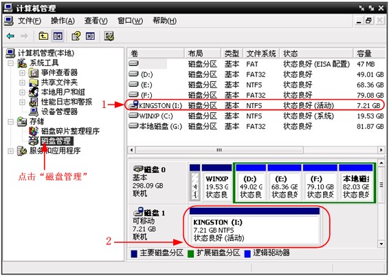
Figure 42: Disk Management on a Computer

Right-click on the red-marked area labeled 1 or 2, and select “Format.” A warning message will appear; select “OK.”

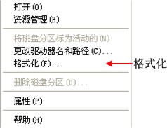
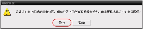
Figure 4 Figure 3: Warning about formatting a USB flash drive

In the formatting window that appears, set the file system to FAT32 and the allocation unit size to 4096. Check the “Perform quick format” box to perform a quick format. Click “OK,” and then select “OK” in the warning dialog that appears.

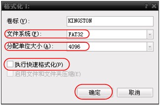
Figure 4: USB Drive Formatting Settings

Formatting in progress

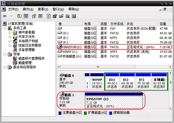
Figure 4, Figure 5: Formatting a USB flash drive

Check whether the USB drive has been formatted with the FAT32 file system and a 4K allocation unit size.

Formatting Using Minitool Partition Wizard

Software download link: http://www.partitionwizard.com/free-partition-manager.html

Note: There are many formatting programs available on the market; this manual uses Minitool Partition Wizard as an example.

Connect the USB flash drive to the computer.

Open the Minitool Partition Wizard software.

Click “Reload Disk” in the drop-down menu in the upper-left corner or press F5 on your keyboard to load the USB drive. The red labels 1 and 2 on the right display information about the USB drive.

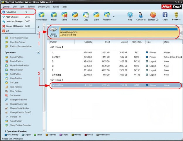
Fig. 4–Fig. 6: Inserting a USB flash drive

Right-click on the red-marked area labeled 1 or 2, and select “Format.”

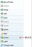
Figure STYLEREF 1 s4SEQ Figure * ARABIC s 17: Software-Formatted USB Drive Warning

In the formatting window that appears, set the file system to FAT32, set the allocation unit size to 4096, and click OK.

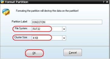
Figure 4, Figure 8: Settings for Formatting a USB Drive Using Software

Click “Apply” in the menu at the top left. A warning will pop up; click “Yes” to begin formatting.

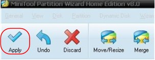
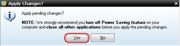
Figure STYLEREF 1 s4SEQ Figure * ARABIC s 19: The software is formatting the USB drive

Proses Pemformatan

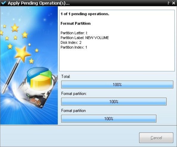
Figure 4, Figure 10: Formatting Process

The USB drive was successfully formatted.

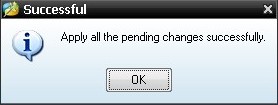
Figure 4, Figure 11: Formatting Successful

How to Configure Assistive System Features

● Konfigurasi

Press the Utility button, select “Functions” from the right-hand menu, and select “Configuration” from the left-hand menu.

The menu descriptions are as shown in the table below:

Function Menu	Pengaturan	Note
Fitur	konfigurasi	Open the configuration menu
Kunci Keypad		When the Lock button is pressed, pressing any other button will have no effect; to unlock, first press the “Trigger Menu” button in the trigger control area, then press the “Force” button. Repeat this sequence three times.
Tentang kami		Display the version number and serial number

● Tampilan

Press the Utility button, select “Functions” from the right-hand menu, and select “Display” from the left-hand menu.

The menu is described in the table below:

Function Menu	Pengaturan	Note
Fitur	Tampilan	Bring up the display menu
Backlight	0 – 100%	Rotate the universal knob to adjust the backlight brightness
kisi		Press the menu button on the right to switch between grid styles.
Menu Hours	Turn off in 5 to 30 seconds	Rotate: General—Set the time after which the left and right menus automatically disappear

● Calibration

Press the Utility button, select Utility from the menu on the right, and select Calibration from the menu on the left.

The menu descriptions are as shown in the table below:

Function Menu	Note
Function Calibration	Access the calibration menu
Kalibrasi mandiri	Have the machine perform a self-calibration
Pengaturan Pabrikan	Kembalikan Pengaturan Pabrik
Inspeksi Penyelidik	Check whether the probe compensation is working properly

Kalibrasi otomatis:
The autocalibration procedure maximizes the oscilloscope’s accuracy at the ambient temperature. If the ambient temperature changes by 5°C or more, you should perform the autocalibration procedure to achieve the highest accuracy.
Before performing autocalibration, disconnect any probes or leads from the input connectors. Press the Utility key, select “Function” from the menu on the right, and the function options menu will appear on the left side of the screen. Select “Calibration,” and once you are ready, select “Auto-Calibration” from the menu on the right to start the instrument’s auto-calibration procedure.

Probe Check:
Used to verify whether probe compensation is proper. There are three possible outcomes: overcompensation, proper compensation, and undercompensation. Users should adjust the probe compensation based on the results to achieve optimal compensation. The procedure is as follows:

Connect the probe to CH1 and set the probe attenuation factor to the maximum;

Press the Utility button, select “Functions” from the menu on the right, and select “Calibration” from the menu on the left;

Select “Probe Check” from the menu on the right, and a probe check prompt will appear on the screen;

In the menu on the right, press “Probe Check” again to start the probe check. The results will be displayed after 3 seconds; press any key to exit.

● Save
: You can save oscilloscope waveforms, settings, or screen images. See “How to Save and Recall” on page 25.

● Upgrade

You can update the instrument’s firmware using a USB storage device connected to the front-panel USB port. See “How to Update the Instrument’s Firmware” on page 33.

How to Update Instrument Firmware

You can update the instrument’s firmware using a USB storage device connected to the front-panel USB port.

USB Storage Device Requirements: Insert the USB storage device into the front-panel USB port. If the icon appears in the upper-right corner of the screen, the USB drive has been successfully recognized. If the system does not recognize the USB drive, please format it according to the method described in P Drive Requirement 27, and then try again.

Note: Updating the instrument’s firmware is a sensitive operation. To prevent damage to the instrument, do not turn off the power or disconnect the USB storage device during the update process.

To update the instrument’s firmware, follow these steps:

Press the Utility button, select “Functions” from the right-hand menu, select “Configuration” from the left-hand menu, and then select “About” from the right-hand menu. View the instrument model and current version number.

Access our website on your PC to check if an updated firmware version is available for your model. Download the firmware file to your PC. The firmware file is always named “Scope.update.” Copy this firmware file to the root directory of a USB storage device.

Insert the USB storage device into the USB port on the front panel of the instrument.

Press the Utility button, select “Utility” from the menu on the right, and select “Update” from the menu on the left.

Click Start in the menu on the right, and the screen will display the upgrade instructions.

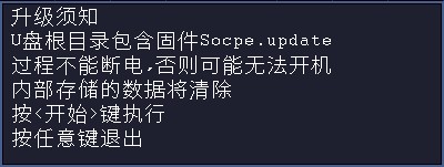
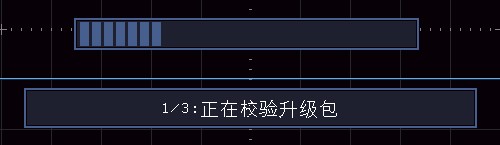
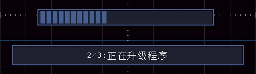
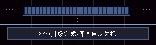
Click Start again in the right-hand menu; the following screens will appear in sequence. The upgrade process may take up to 3 minutes. Once the upgrade is complete, the instrument will automatically shut down.

Nyalakan perangkat dengan menekan tombol daya.

How to Perform Automatic Measurements

Press the “Measure” button to start automatic measurement. There are 30 types of measurements available, and up to 8 measurement types can be displayed in the lower-left corner of the screen.

30 types of automatic measurements include: period, frequency, average, peak-to-peak, root mean square (RMS), maximum, minimum, top value, bottom value, amplitude, overshoot, pre-shoot, rise time, fall time, positive pulse width, negative pulse width, positive duty cycle, negative duty cycle, delay A-> B, Delay A-> B, Period RMS, Cursor RMS, On-Screen Duty Cycle, Phase, Number of Positive Pulses, Number of Negative Pulses, Number of Rising Edges, Number of Falling Edges, Area, and Period Area.

The description of the automatic measurement function menu is as shown in the table below:

Function Menu	Pengaturan	Note
Add CH1	Measurement Types (Left Menu)	Press this button to display the left-hand menu, turn the “General” knob to select the type of measurement, and then press this button to add a CH1 measurement item.
Add CH2	Measurement Type (Left Menu)	Press this button to display the menu on the left, turn the “General” knob to select the measurement type, and then press this button to add a CH2 measurement item.
Potret	Turn off CH1 CH2	Close Measurement Snapshot Show All Measurements for CH1 Show All Measurements for CH2
Delete	Measurement Types (Left-hand Menu)	Press this button to display the list on the left, turn the “General” knob to select the measurement item you want to delete, and then press this button again to delete it.
Hapus Semua		Delete All Measurements

Pengukuran:

The waveform channel must be turned on to perform measurements. Automatic measurements cannot be performed on stored waveforms, calculated waveforms from dual waveforms, or when the trigger mode is set to video. During slow scan, the period and frequency cannot be measured.

To measure the period and frequency of the signal on Channel CH1, follow these steps:

Press the Measure button to display the automatic measurement menu on the right side of the screen.

Click “Add CH1” in the menu on the right.

The measurement type menu appears on the left side of the screen; turn the “General” knob to select the “Period” option.

In the menu on the right, click “Add CH1” to complete the cycle setup.

In the Type menu on the left side of the screen, turn the General knob to select the Frequency option.

In the menu on the right, select “Add CH1” to complete the frequency settings. The measurement values will automatically appear
in the lower-left corner of the screen. See Figure 412:

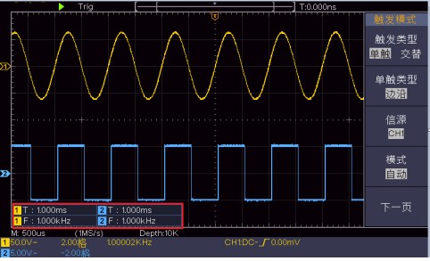
Figure 4, Figure 12: Automatic Measurement

Automatic Measurement of Voltage Parameters

Voltage parameters that an oscilloscope can measure automatically include average, peak-to-peak, root mean square (RMS), maximum, minimum, top, bottom, amplitude, overshoot, pre-shoot, period RMS, and cursor RMS. The figure below illustrates the physical meanings of these voltage parameters.

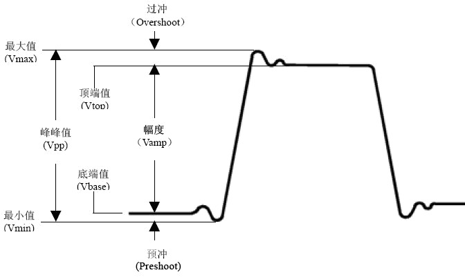
Figure 4, Figure 13: Schematic of voltage parameter definitions (flat-top with a pulse signal)

Average: The arithmetic mean of the entire waveform or the selected region.

Peak-to-Peak (Vpp): The voltage between the peak of the waveform and its trough.

Root Mean Square (Vrms): The precise “root mean square” voltage across the entire waveform or the selected region.

Maximum Value (Vmax): The voltage from the peak of the waveform to GND (ground).

Minimum Value (Vmin): The voltage from the lowest point of the waveform to GND (ground).

Peak Value (Vtop): The voltage from the top of the waveform to GND (ground).

Base Voltage (Vbase): The voltage from the flat bottom of the waveform to GND (ground).

Amplitude (Vamp): The voltage value from the peak to the trough of the waveform.

Overshoot: The ratio of the difference between the waveform’s maximum value and its peak value to the amplitude.

Preshoot: The ratio of the difference between the waveform’s minimum and the bottom value to the amplitude.

Cycle RMS: Calculates the root mean square value of the first complete cycle of the waveform.

Cursor RMS: Calculates the true root mean square (RMS) of the waveform data between the selected start and end points.

An
oscilloscope with automatic time measurement capabilities can automatically measure a signal’s period, frequency, rise time, fall time, positive pulse width, negative pulse width, positive duty cycle, negative duty cycle, delay A-> B, delay A-> B, on-screen duty cycle, and phase.

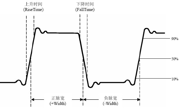
Figure 414: Schematic of Time Parameter Definitions

Rise Time: The time it takes for the waveform amplitude to rise from 10% to 90%.

Fall Time: The time it takes for the waveform amplitude to decrease from 90% to 10%.

Positive Pulse Width (+Width): The pulse width of a positive pulse at 50% amplitude.

Negative Pulse Width (-Width): The pulse width of a negative pulse at 50% amplitude.

Positive Duty Cycle (+Duty): The ratio of the positive pulse width to the period.

Negative Duty Cycle (-Duty): The ratio of the negative pulse width to the period.

Delay A-> B: The delay in channels A and B relative to the rising edge.

Delay A-> B: The delay in channels A and B relative to the falling edge.

Screen Duty Cycle: The ratio of the duration of the positive pulse to the total period.

Phase: The rising edge of the first signal is compared with the rising edge of the second signal to calculate the phase angle difference between signals in different channels. The phase angle difference is calculated as (channel delay ÷ period) × 360°.

Other measurements:

Number of Positive Pulses: The number of positive pulses within the waveform region that rise above the middle crossover reference.

Number of Negative Pulses: The number of negative pulses within the waveform region that fall below the middle cross-reference.

Number of Rising Edges: The number of times the waveform transitions from a low reference value to a high reference value within the waveform region.

Number of falling edges: The number of times the waveform transitions from a high reference value to a low reference value within the waveform region.

Area: The area of the entire waveform within the screen, measured in volt-seconds. Areas measured above the zero reference (i.e., vertical offset) are positive, while those measured below the zero reference are negative; the measured area is the algebraic sum of the areas of the entire waveform within the screen.

Cycle Area: The area of the first cycle of the screen waveform, measured in volt-seconds. The area above the zero reference (i.e., the vertical offset) is positive, while the area below the zero reference is negative; the measured area is the algebraic sum of the areas of all cycles. Note: When the screen waveform does not span a full cycle, the measured cycle area is zero.

How to Perform Cursor Measurements

Press the Cursor key to display the cursor measurement menu on the screen. Press the Cursor key again to turn off the cursor.

Cursor Measurement in Normal Mode:
The Cursor Measurement menu is described in the table below:

Function Menu	Pengaturan	Note
Tipe	Voltage, Time, Time & Voltage, Auto Cursor	Display voltage measurement cursors and menus Display time measurement cursors and menus Display time and voltage measurement cursors and menus The position of the horizontal cursor is automatically set to the intersection of the vertical cursor and the waveform
Measurement Selection (Type: Time & Voltage)	Time Voltage	Select the vertical cursor line. Select the horizontal cursor line.
Window Selection (Enter Waveform Zoom)	Main Window, Secondary Window	Main Measurement Window | Secondary Measurement Window
Cursor Line	a b ab	Turn the General knob to move cursor line a. Turn the General knob to move cursor line b. Link a and b; turning the General knob moves both cursors simultaneously.
sumber	CH1/CH2	Select the waveform channel to be measured by the cursor

To perform cursor measurements of both time and voltage on Channel CH1 simultaneously, follow these steps:

Press the Cursor panel button to bring up the cursor measurement menu.

In the menu on the right, select CH1 as the source.

Select the first menu item in the right-hand menu to switch the display type to “Time & Voltage.” The screen will display two blue dashed lines vertically and two blue dashed lines horizontally. The cursor increment window, located at the bottom left of the waveform display area, shows the cursor reading.

In the right-hand menu, select “Time” under “Measurement Selection” to enable both vertical cursors. When “a” is selected under “Cursor Lines” in the right-hand menu, turning the “General” knob moves the “a” cursor to the left or right. When “b” is selected, turning the “General” knob moves the “b” cursor.

In the menu on the right, select “Measurement” and set it to “Voltage” to enable the two horizontal cursors. Select “a” or “b” under “Cursor Line,” then turn the “General” knob to move them.

Press the HOR key to enter waveform zoom mode. Press the Cursor panel key to bring up the right-side cursor measurement menu, and switch the Window Selection to Main Window or Subwindow to display the cursor line in the main window or subwindow.

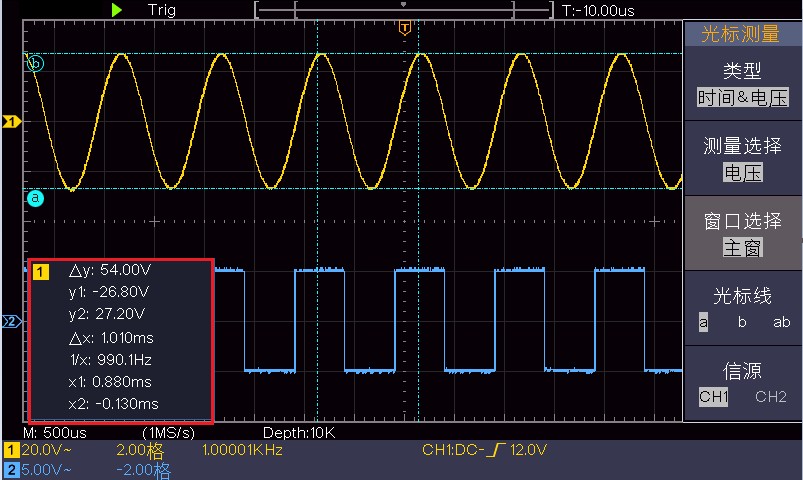
Figure 4, Figure 15: Waveforms Measured Using Time and Voltage Cursors

Automatic Cursor

In automatic cursor mode, the horizontal cursor is automatically positioned at the intersection of the vertical cursor and the waveform.

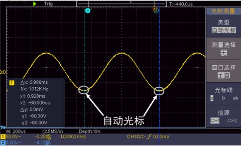
Cursor Measurements in FFT Mode:

In FFT mode, press the Cursor key to display the cursor measurement function menu on the screen. The menu descriptions are shown in the table below:

Function Menu	Pengaturan	Note
Tipe	Amplitude, Frequency, Frequency & Amplitude, Auto Cursor	Display the amplitude measurement cursor and menu. Display the frequency measurement cursor and menu. Display the frequency and amplitude measurement cursors and menus. The position of the horizontal cursor is automatically set to the intersection of the vertical cursor and the waveform.
Measurement Options (Type: Frequency & Amplitude)	Frequency, Amplitude	Select the vertical cursor line. Select the horizontal cursor line.
Pilihan Jendela	Main Window Secondary Window	Main Measurement Window | FFT Subwindow
Cursor Line	a b ab	Turn the General knob to move cursor line a. Turn the General knob to move cursor line b. Link a and b; turning the General knob moves both cursors simultaneously.
sumber	MathFFT	Display Source

To perform Math FFT amplitude and frequency cursor measurements simultaneously, follow these steps:

Press the Math key to display the waveform calculation menu on the right, then select FFT for Type.

Press the Cursor panel button to bring up the cursor measurement menu.

In the right-hand cursor measurement menu, select “Window Selection” as “Subwindow,”

Select the first menu item in the right-hand menu to switch the display type to “Frequency & Amplitude.” The subwindow will display two blue dashed lines vertically and two blue dashed lines horizontally. The cursor increment window, located at the bottom left of the waveform display area, shows the cursor reading.

In the right-hand menu, select “Measurement” and set it to “Frequency” to enable both vertical cursors. When “a” is selected under “Cursor Lines” in the right-hand menu, turning the “General” knob moves the a cursor to the left or right. When “b” is selected, turning the “General” knob moves the b cursor.

In the menu on the right, select “Measurement” and set it to “Amplitude” to select the two horizontal cursors. Select “a” or “b” under “Cursor Line,” then turn the “General” knob to move them.

In the right-hand cursor measurement menu, select “Window Selection” as “Main Window” to display the cursor line in the main window.

How to Use the Execute Key

The function buttons include Auto Setup, Run/Stop, and Copy.

[Auto Setup] Button

Automatically sets the instrument’s various control parameters to produce a waveform suitable for observation. Press the Auto Setup button, and the oscilloscope will quickly and automatically measure the signal.
The Auto Setup functions are listed in the table below:

Barang Fungsional	Pengaturan
Vertical Coupling	Sekarang
Channel Coupling	Sekarang
Vertical Gears	Shift to the appropriate gear
Perpindahan horizontal	Centered or ±2 spaces
Horizontal Gears	Shift to the appropriate gear
Tipe Pemicu	Edge or Video
Sumber Pemicu	CH1 or CH2
Kopling Pemicu	Arus searah
Pemicu Kemiringan	Sekarang
Level Pemicu	The point where the signal is 3/5 of its maximum
Metode Pemicu	secara otomatis
Tampilan Pilihan	YT
Force Run	berhenti
Terbalik	Penyelesaian
Waveform Zoom	Exit

Automatically Determine Waveform Type

There are five types: sine waves, square waves or pulse waves, video signals, DC levels, and unknown signals.

A waveform type prompt pops up on the screen, and the corresponding right-side menu appears.

Waveform	Right-side menu items
Gelombang sinus	Multi-cycle, Single-cycle, FFT, Clear Auto Settings
Square Wave or Pulsed Wave	Multi-cycle, Single-cycle, Rising Edge, Falling Edge, Clear Auto Settings
Video Sinyal	Type (Row/Field), Odd Field, Even Field, Specified Row, Cancel Auto Settings
DC voltage or unknown signal	Cancel Auto Settings

Explanation of Selected Terms:

Multiple Cycles: Displays multiple waveform cycles.

Single Cycle: Displays 1 to 2 waveform cycles.

FFT: Switch to FFT display.

Rising Edge: Displays a single rising edge of a square wave.

Falling Edge: Displays a single falling edge of a square wave.

Cancel Auto Settings: Return to the previous menu and signal information.

Note: When using the automatic waveform setup function, the frequency of the signal under test must be at least 20 Hz, and the amplitude must be at least 5 mV. If these conditions are not met, the automatic waveform setup function may not work.

[Run/Stop] Button
: Starts and stops waveform sampling.

Note: In the stopped state, the vertical scale and horizontal time base can be adjusted within a certain range, which is equivalent to expanding the signal horizontally or vertically. When the horizontal time base is 50 ms or less, it can be expanded downward by 4 steps.

[Copy] Key
: This key is the shortcut for the “Save” function in the Function Panel menu. Pressing this key is equivalent to selecting “Save” from the Save menu. It saves waveforms, settings, or screen images based on the save type selected in the Save menu. For details, see “How to Save and Recall” on page 25.

5. Communication with Host Computer Software

The oscilloscope supports communication with the host computer via a USB interface. The Oscilloscope host software installed on the computer provides functions such as storing, analyzing, and displaying measurement data from the oscilloscope, as well as remote control.

For specific instructions on how to use the Oscilloscope PC software, press the F1 key on the software interface to view the built-in help documentation.

The following explains how to connect to a computer using the USB port.

Install the software: Install the Oscilloscope PC software from the included CD on your computer.

Connection: Use a USB cable to connect the USB Device port on the rear panel of the oscilloscope to a USB port on the computer.

Installing the Driver: After running the Oscilloscope PC software on your computer, press the F1 key to open the built-in help documentation, and follow the steps under the heading “I. Connecting the Device to the PC” to install the driver.

Host Computer Communication Port Settings: Open the Oscilloscope software, click “Transfer” in the menu bar, select “Port Settings,” and in the settings dialog box, select “USB” as the communication port. Once the connection is successful, the connection status indicator in the lower-right corner of the software interface will turn green.

6. Contoh Aplikasi

Example 1: Measuring Simple Signals

Observe an unknown signal in the circuit and quickly display and measure the signal’s frequency and peak-to-peak value.

To display this signal quickly, follow these steps:

Set the probe menu attenuation factor to 10X and set the switch on the probe to 10X (see “How to Set the Probe Attenuation Factor” on page 10).

Connect the probe for Channel 1 to the point on the circuit under test.

Press the “Auto Setup” button.

The oscilloscope will automatically adjust the settings to optimize the waveform display. From there, you can further adjust the vertical and horizontal scales until the waveform display meets your requirements.

Perform an automatic measurement

The oscilloscope can automatically measure most display signals. To measure the period and frequency of the signal on CH1, follow these steps:

Press the Measure button to display the automatic measurement menu on the right side of the screen.

Click “Add CH1” in the menu on the right.

The measurement type menu appears on the left side of the screen; turn the “General” knob to select the “Period” option.

In the menu on the right, click “Add CH1” to complete the cycle setup.

In the type menu on the left side of the screen, turn the “General” knob to select the “Frequency” option.

In the menu on the right, select “Add CH1” to complete the frequency selection.
The measurement values will automatically appear in the lower-left corner of the screen. See Figure 61.

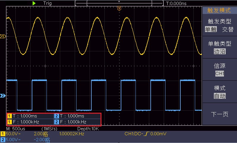
Figure 6, Figure 1: Automatic Waveform Measurement

Example 2: Measuring the Gain of an Amplifier in a Circuit

Set the probe menu attenuation factor to 10X and set the switch on the probe to 10X (see “How to Set the Probe Attenuation Factor” on page 10).

Connect the oscilloscope’s CH1 channel to the circuit’s input terminal and the CH2 channel to the output terminal.

petunjuk:

Press the “Auto Setup” button. The oscilloscope automatically adjusts the waveforms on both channels for proper display.

Press the Measure button to display the automatic measurement menu on the right side of the screen.

Click “Add CH1” in the menu on the right.

The measurement type menu appears on the left side of the screen; turn the “General” knob to select the “Peak-to-Peak” option.

In the menu on the right, press “Add CH1” to complete the peak-to-peak measurement for CH1.

In the menu on the right, press “Add CH2” to complete the peak-to-peak measurement for CH2.

Read the peak-to-peak values for CH1 and CH2 from the display area in the lower-left corner of the screen. See Figure 62.

Use the following formula to calculate the amplifier gain.

Gain = Output Signal / Input Signal

Gain (dB) = 20 × log(gain)

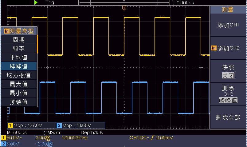
Figure 6, Figure 2: Gain Measurement Waveforms

Example 3: Capturing a Single Signal

The ability to conveniently capture non-periodic signals, such as pulses and glitches, is a key advantage and feature of Digital Oscilloscopes. To capture a one-shot signal, you first need some prior knowledge of the signal in order to set the trigger level and trigger edge. For example, if the pulse is a TTL-level logic signal, the trigger level should be set to 2 volts, and the trigger edge should be set to rising-edge trigger. If the nature of the signal is uncertain, you can first observe it using automatic or standard trigger modes to determine the appropriate trigger level and trigger edge.

Langkah-langkahnya adalah sebagai berikut:

Set the probe menu attenuation factor to 10X and set the switch on the probe to 10X (see “How to Set the Probe Attenuation Factor” on page 10).

Adjust the vertical and horizontal range knobs to set appropriate vertical and horizontal ranges for the signal being observed.

Press the “Sample” button to display the sampling menu on the right.

In the menu on the right, select “Peak Detection” as the acquisition mode.

Press the “Trigger Menu” button to display the trigger menu on the right.

In the menu on the right, select “Single Touch” as the trigger type.

In the menu on the right, select “Edge” as the single-touch type.

In the menu on the right, select CH1 as the source.

In the menu on the right, click “Next Page” and select “DC” for “Coupling.”

In the menu on the right, select “Slope” as “Up.”

Turn the Trigger Level knob to adjust the trigger level to the midpoint of the signal under test.

If “Ready” is not displayed in the trigger status indicator at the top of the screen, press the Run/Stop button to start data acquisition. Wait for a signal that meets the trigger conditions to appear. If a signal reaches the set trigger level, one sample is taken and displayed on the screen. This feature makes it easy to capture sporadic events, such as sudden glitches with large amplitudes: Set the trigger level to just above the normal signal level, press the Run/Stop button to begin waiting, and when a glitch occurs, the instrument will automatically trigger and record the waveform for a period before and after the trigger. By rotating the “Horizontal Offset” knob in the horizontal control area on the panel to adjust the horizontal offset of the trigger position, you can achieve negative-delay triggers of varying lengths, making it easier to observe the waveform before the glitch occurs. See Figure 63.

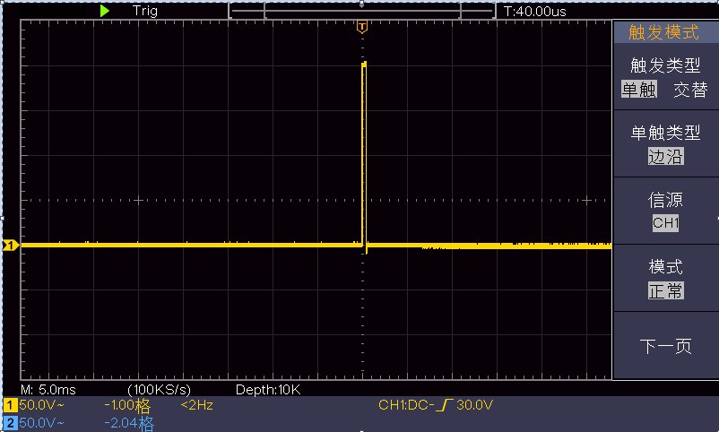
Figure 6, Figure 3: Capturing a Single Signal

Example 4: Analyzing Signal Details

Observing a Noisy Signal

The signal is being interfered with by noise, which may cause the circuit to malfunction. To analyze the noise in detail, follow these steps:

Press the “Sample” button to display the sampling menu on the right.

In the menu on the right, select “Peak Detection” as the acquisition mode.

At this point, the screen displays a waveform containing random noise. Especially when the time base is set to a slow setting, peak detection allows you to observe the noise spikes and glitches present in the signal. See Figure 64.

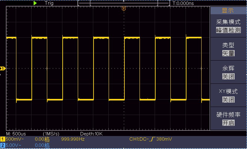
Figure 6, Figure 4: Waveforms of signals containing noise

Memisahkan Sinyal dari Derau

When analyzing signal waveforms, it is necessary to remove noise. To reduce the random noise displayed on the oscilloscope, follow these steps:

Press the “Sample” button to display the sampling menu on the right.

In the menu on the right, select “Average” as the acquisition mode.

In the left-hand menu, turn the “General” knob to select different averaging counts and observe how the waveform appears after averaging.

After averaging, the random noise is reduced and the signal details become easier to observe. In the figure below, once the noise is removed, glitches on the rising and falling edges of the signal become visible. See Figure 65.

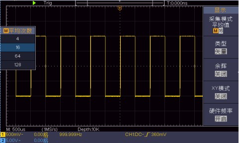
Figure 6, Figure 5: Waveforms of the denoised signal

Example 5: Applications of the X–Y Function

View an example of the phase difference
between two-channel signals: the phase change introduced by a circuit network as the test signal passes through it.
Connect the oscilloscope to the circuit and monitor the circuit’s input and output signals.

To view the circuit’s inputs and outputs in an X-Y plot, follow these steps:

Set the probe menu attenuation factor to 10X and set the switch on the probe to 10X (see “How to Set the Probe Attenuation Factor” on page 10).

Connect the probe for Channel 1 to the network’s input, and connect the probe for Channel 2 to the network’s output.

Press the “Auto Setup” button, and the oscilloscope will enable the signals on both channels and display them on the screen.

Adjust the vertical gain knob so that the amplitudes of the two signals are approximately equal.

Press the “Sampling” button on the panel to bring up the menu on the right.

In the menu on the right, select “XY Mode” and set it to “On.” The oscilloscope will display the network’s input-output characteristics in Lissajous figure mode.

Adjust the “Vertical Range” and “Vertical Offset” knobs to optimize the waveform.

Use the elliptical oscillogram method to observe and calculate the phase difference. See Figure 66.

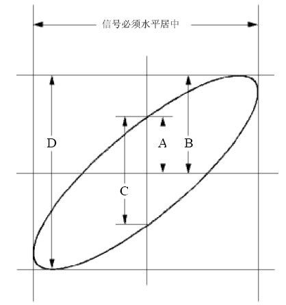
Figure 6: Lissajous figures

Based on sin q = A/B or C/D, where q is the phase difference angle between the channels, and the definitions of A, B, C, and D are shown in the figure above. Therefore, the phase difference angle can be derived as follows: q = ± arcsin (A/B) or ± arcsin (C/D). If the major axis of the ellipse lies in Quadrants I or III, then the calculated phase difference angle should lie in Quadrants I or IV, that is, within the range (0 to π/2) or (3π/2 to 2π). If the major axis of the ellipse lies in quadrants II or IV, then the calculated phase difference angle should lie in quadrants II or III, that is, within the range (π/2 to π) or (π to 3π/2).

Example 6: Video Signal Trigger

Observe the video circuitry in a television set, use video triggering to obtain a stable video output signal for display.

Video Field Trigger

To trigger this in the video feed, follow these steps:

Press the “Trigger Menu” button to display the trigger menu on the right.

In the menu on the right, select “Single Touch” as the trigger type.

In the menu on the right, select “Video” as the single-touch type.

In the menu on the right, select CH1 as the source.

In the menu on the right, select NTSC as the video standard.

Click “Next Page,” then select “Synchronize as Field” from the menu on the right.

Adjust the Vertical Range, Vertical Offset, and Horizontal Range knobs to obtain the desired waveform display.

See Figure 67:

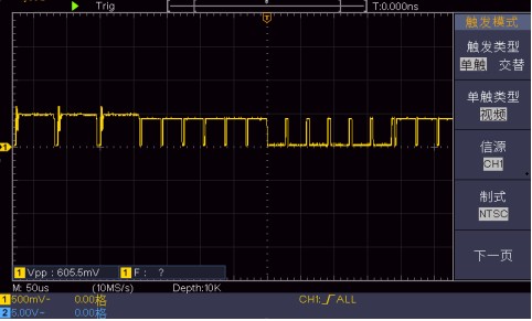
Fig. 6, Fig. 7: Video-frame triggering

Penyelesaian masalah

If the oscilloscope screen remains blank with no display after pressing the power switch, please follow these steps:
• Check to make sure the power cord is securely plugged in.
• After completing the above checks, restart the instrument.
• If the product still does not function properly, please contact us so we can assist you.

If no signal waveform appears on the screen after signal acquisition, follow these steps:
• Check whether the probe is properly connected to the signal cable.
• Check whether the signal cable is properly connected to the BNC connector (i.e., the channel connector).
• Check whether the probe is properly connected to the device under test.
• Check whether the device under test is generating a signal(You can connect a channel that is generating a signal to the problematic channel to pinpoint the issue.)
• Try acquiring the signal again.

The measured voltage amplitude is 10 times greater or 10 times less than the actual value.
Check whether the attenuation factor in the channel settings menu matches the actual probe attenuation ratio (see “How to Set the Probe Attenuation Factor” on page 10).

A waveform is displayed, but it does not stabilize.
• Check whether the “Source” option in the Trigger Mode menu matches the signal channel actually in use.
• Check the “Trigger Type” option: For general signals, use edge triggering; for video signals, use video triggering. If Alternate Trigger is selected, adjust the trigger levels for both channels to appropriate settings. The waveform will only display stably when the appropriate trigger mode is applied.

Pressing the Run/Stop key produces no display.
Check whether the trigger mode in the Trigger Mode menu is set to Normal or Single, and whether the trigger level is outside the waveform range. If so, center the trigger level or set the trigger mode to Auto. Alternatively, press the Autoset key to automatically complete these settings.

When set to average sampling in acquisition mode (see “How to Set Acquisition/Display” on p. 24), or when the afterglow duration is set to a long value in the display settings (see “Afterglow” on p. 24), the display speed slows down.
Ini normal.

Technical Specifications Unless otherwise specified, all technical specifications apply to probes and digital oscilloscopes with the attenuation switch set to 10X. To meet these specifications, the oscilloscope must first satisfy the following two conditions: • The instrument must operate continuously for at least 30 minutes at the specified operating temperature. • If the operating temperature varies by 5°C or more, you must open the system function menu and perform the “Self-Calibration” procedure (see “How to Perform Self-Calibration” on page 11).

With the exception of specifications marked as “typical,” all specifications used are guaranteed.

Fitur	Fitur	Fitur	Note	Note
Memasukkan	Kopling masukan	Kopling masukan	DC, AC, Grounding	DC, AC, Grounding
Memasukkan	Impedansi masukan	Impedansi masukan	1 MΩ ± 2%, in parallel with 20 pF ± 5 pF	1 MΩ ± 2%, in parallel with 20 pF ± 5 pF
Memasukkan	Probe Attenuation Coefficient	Probe Attenuation Coefficient	1X, 10X, 100X, 1000X	1X, 10X, 100X, 1000X
Memasukkan	Tegangan Input Maksimum	Tegangan Input Maksimum	400 V (DC + AC peak)	400 V (DC + AC peak)
Memasukkan	Isolasi antar saluran	Isolasi antar saluran	50 Hz: 100 : 1 10 MHz: 40 : 1	50 Hz: 100 : 1 10 MHz: 40 : 1
Memasukkan	Time Delay Between Channels (Typical)	Time Delay Between Channels (Typical)	150ps	150ps
Memasukkan	Waveform Interpolation	Waveform Interpolation	(sinx)/x	(sinx)/x
Memasukkan	Maximum storage depth	Maximum storage depth	10K	10K
Memasukkan	Time-base accuracy	Time-base accuracy	± 100 ppm	± 100 ppm
Memasukkan	Time Interval (△T) Measurement Accuracy (DC–100 MHz)	Time Interval (△T) Measurement Accuracy (DC–100 MHz)	Single measurement: ±(1 sampling interval + 100 ppm × reading + 0.6 ns) > 16 averages: ±(1 sampling interval + 100 ppm × reading + 0.4 ns)	Single measurement: ±(1 sampling interval + 100 ppm × reading + 0.6 ns) > 16 averages: ±(1 sampling interval + 100 ppm × reading + 0.4 ns)
Vertikal	Analog-to-Digital Converter (A/D)	Analog-to-Digital Converter (A/D)	8-bit resolution, with simultaneous sampling on two channels.	8-bit resolution, with simultaneous sampling on two channels.
Vertikal	Sensitivity (V/grid) Range	Sensitivity (V/grid) Range	5 mV/div hingga 5 V/div	5 mV/div hingga 5 V/div
Vertikal			NDS1202S	200 MHz
Vertikal	One-Way Bandwidth	One-way bandwidth	Lebar pita penuh	Lebar pita penuh
Vertikal	Low-Frequency Response (AC-Coupled, -3 dB)	Low-Frequency Response (AC-Coupled, -3 dB)	≥10 Hz (on the BNC connector)	≥10 Hz (on the BNC connector)
Vertikal	Akurasi Penguatan DC	Akurasi Penguatan DC	± 3%	± 3%
Vertikal	DC Measurement Accuracy (Average Value, Sampling Method)	DC Measurement Accuracy (Average Value, Sampling Method)	After averaging ≥16 captured waveforms, the voltage difference (△V) between any two points on the waveform is: ±(3% of the reading + 0.05 divisions).	After averaging ≥16 captured waveforms, the voltage difference (△V) between any two points on the waveform is: ±(3% of the reading + 0.05 divisions).
Vertikal	Turn Waveform Inversion On/Off	Turn Waveform Inversion On/Off	Turn Waveform Inversion On/Off	Turn Waveform Inversion On/Off
Measurement	Pengukuran Kursor	Pengukuran Kursor	Voltage difference between markers (△V), time difference between markers (△T)	Voltage difference between markers (△V), time difference between markers (△T)
Measurement	Pengukuran Otomatis	Pengukuran Otomatis	Period, Frequency, Average, Peak-to-Peak, Root Mean Square, Maximum, Minimum, Top Value, Bottom Value, amplitude, overshoot, pre-overshoot, rise time, fall time, positive pulse width, negative pulse width, positive duty cycle, negative duty cycle, delay A→B, delay A→B, period RMS, cursored RMS, duty cycle, phase	Period, Frequency, Mean, Peak-to-Peak, Root Mean Square, Maximum, Minimum, Top Value, Bottom Value, amplitude, overshoot, pre-shoot, rise time, fall time, positive pulse width, negative pulse width, positive duty cycle, negative duty cycle, delay A-> B, delay A-> B, period RMS, cursor RMS, duty cycle, phase
Measurement	Operasi Matematika	Operasi Matematika	Addition, Subtraction, Multiplication, Division, FFT	Addition, Subtraction, Multiplication, Division, FFT
Measurement	Save Waveform	Save Waveform	16 sets of waveforms	16 sets of waveforms
Measurement	Li Shayou’s Diagram	Bandwidth	Lebar pita penuh	Lebar pita penuh
Measurement	Li Shayu’s Graphics	Perbedaan fase	± derajat 3	± derajat 3
Antarmuka Komunikasi	USB 2.0, supports USB flash drive storage	USB 2.0, supports USB flash drive storage	USB 2.0, supports USB flash drive storage	USB 2.0, supports USB flash drive storage
Penghitung Frekuensi	Bantuan	Bantuan	Bantuan	Bantuan

Pelatuk:

Fitur	Fitur	Fitur	Note
Trigger Level Range	Intern	Intern	±5 grid units from the center of the screen
Trigger Level Accuracy (Typical): This accuracy applies to signals with rise and fall times of ≥20 ns.	Intern	Intern	±0.3 grid units
Trigger Displacement	Depending on the storage depth and time base setting	Depending on the storage depth and time base setting	Depending on the storage depth and time base setting
Scope of Exemption	100 ns to 10 s	100 ns to 10 s	100 ns to 10 s
Set the level to 50% (typical)	Operation under conditions where the input signal frequency is ≥ 50 Hz	Operation under conditions where the input signal frequency is ≥ 50 Hz	Operation under conditions where the input signal frequency is ≥ 50 Hz
Edge Trigger	Lereng	Atas, Bawah	Atas, Bawah
Video Trigger	Signaling System	Supports NTSC, PAL, and SECAM broadcast systems with any field or line frequency	Supports NTSC, PAL, and SECAM broadcast systems with any field or line frequency
Video Trigger	Rentang Frekuensi Operasi	The line range is 1–525 (NTSC) and 1–625 (PAL/SECAM)	The line range is 1–525 (NTSC) and 1–625 (PAL/SECAM)

display:

Fitur	Note
Tampilan Jenis	7- to 8-inch color LCD display
Resolusi layar	800 horizontal × 480 vertical pixels
Warna tampilan	65536 colors, TFT

Probe Compensator Output:

Fitur	Note
Output Voltage (Typical)	Approximately 5 V, peak-to-peak, with a load of ≥ 1 MΩ
Frequency (typical)	1 kHz square wave

Sumber Daya listrik:

Fitur	Note
Power Supply Voltage	100–240 VAC RMS, 50/60 Hz, CAT II
Konsumsi daya	Kurang dari 15 W.
Sekering	2 A, Class T, 250 V

Lingkungan Hidup:

Fitur	Note
Suhu	Operating temperature: 0°C to 40°C; Storage temperature: -20°C to +60°C
Kelembaban relatif	≤90%
Tinggi	Operational range: 3000 meters; Non-operational range: 15000 meters
Metode Pendinginan	Konveksi Alami

Spesifikasi Teknik:

Fitur	Note
Ukuran	301 mm (length) × 152 mm (height) × 70 mm (width)
Berat	1.1 kilograms (main unit)

Calibration Interval: The recommended calibration interval is one year.

1.

2. : Attachment

(Images are for reference only; actual product may vary.)

Standard Attachments:	Standard Attachments:	Standard Attachments:	Standard Attachments:	Standard Attachments:
Kabel Listrik	CD	Panduan Cepat	Kabel USB	A Glimpse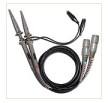
Probe Calibration Pen
Pilih Aksesori:	Pilih Aksesori:	Pilih Aksesori:	Pilih Aksesori:	Pilih Aksesori:
Soft-sided bag

3. : Daily Maintenance and Cleaning

For routine maintenance
, do not store or place the instrument where the LCD screen will be exposed to direct sunlight for extended periods.
Caution: Do not allow aerosols, liquids, or solvents to come into contact with the instrument or the probe, as this may damage them.

Clean and inspect the instrument and probes regularly,
depending on usage. Follow these steps to clean the exterior of the instrument:

1. Use a soft cloth to wipe away any surface dust from the exterior of the device and the probe. When cleaning the LCD screen, be careful not to scratch the transparent LCD protective cover.

2. Wipe the instrument with a soft, damp cloth that does not drip water. Be sure to disconnect the power supply first. You may use a mild detergent or plain water to clean it. Do not use any abrasive chemical cleaners, as they may damage the instrument or the probe.

Warning: Before reconnecting the power, make sure the instrument is completely dry to prevent electrical shorts or even personal injury caused by moisture.